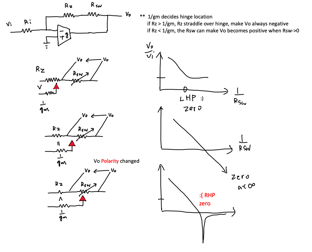
Here g is a transconductance (units A/V), so the amplifier output is a current, not a voltage:
the OTA injects $I_{out}=g\,(V_+-V_-)=-g\,V_x$ into node Vo. Input Ri runs from Vi
to the summing node Vx (– input); feedback Rz + Rsw runs from Vo back to Vx;
Rsw is the swept variable resistor. Let $R_f = R_z + R_{sw}$.
KCL at Vo: $-gV_x=(V_o-V_x)/R_f\Rightarrow V_o=V_x(1-gR_f)$. KCL at Vx: $V_i=V_x(1+gR_i)$. Dividing:
Every product $g R$ = (A/V)(Ω) is dimensionless, so $V_o/V_i$ is unitless. ✔ Ideal limit $g\to\infty$: $V_o/V_i\to -(R_z+R_{sw})/R_i$. Transmission null when $g R_f = 1$ (numerator → 0).
Three regimes of the transconductance g define the three color-coded curves in the plot below. What distinguishes them is where the transmission null ($gR_f=1$) sits relative to the swept resistor.
| Curve | Condition | Vo/Vi | Null location ($gR_f=1$) |
|---|---|---|---|
| Ideal | $g \to \infty$ | $\displaystyle -\frac{R_z+R_{sw}}{R_i}$ | no null (max gain) |
| Critical | $g = 1/R_z$ | $\displaystyle -\frac{R_{sw}}{R_i+R_z}$ | null at $R_{sw}=0$ (edge) |
| Under | $g < 1/R_z$ | $\displaystyle \frac{1-g(R_z+R_{sw})}{1+g\,R_i}$ | null at $R_{sw}=\tfrac1g-R_z>0$ (inside sweep) |
As g drops below $1/R_z$ the null $R_f=1/g$ moves out to a positive $R_{sw}=\tfrac1g-R_z$, so the dip migrates into the visible range (watch the red curve). At exactly $g=1/R_z$ the null sits at $R_{sw}=0$ (the right edge), and for $g\to\infty$ there is no null at all. The red curve's g is set by the g slider; the blue curve is locked to $g=1/R_z$. In the plot you can sweep $x=1/R_{sw}$, $x=1/R_i$, or $x=g$.
| Asymptote / point | Value |
|---|---|
| Ideal @ x→0 | +∞ |
| Finite @ x→0 | +∞ |
| Ideal @ x→∞ | Rz/Ri |
| Finite @ x→∞ | 0 (null) |
Because g is a transconductance, the corrected transfer function is |Vo/Vi| = |1 − g(Rz+Rsw)| / (1 + g·Ri), which is properly unitless. The ideal curve (Rz+Rsw)/Ri grows without bound as Rsw rises (1/Rsw→0) and flattens to Rz/Ri ≈ 0.01 as Rsw→0. The finite curve collapses to the clean Rsw/(Ri+Rz) — a straight slope −1 line on log–log — that plunges to a transmission null (Vo/Vi = 0) at Rsw = 0, i.e. wherever g·Rf = 1. There is no saturation ceiling here; the "saturation at 1/Rz" from earlier revisions was an artifact of the wrong voltage-gain model. At large Rsw the two curves run nearly parallel (both ∝ Rsw), separated only by the factor (Ri+Rz)/Ri = 1 + Rz/Ri.
Sweeping 1/Ri instead (with Rsw fixed): the ideal curve is (Rz+Rsw)/Ri, rising as Ri→0, while the finite curve is Rsw/(Ri+Rz). With the default Rsw = 0 the finite output is identically 0 for every Ri — the whole Ri axis sits on the transmission null, because g·Rf = g·Rz = 1 regardless of Ri. Note: when Ri = 0 the ideal gain diverges (input shorted to the virtual-ground node), so it clips at the top of the chart.
Sweeping g (with Ri, Rsw fixed): the actual curve |Vo/Vi|(g) = |1 − g·Rf| / (1 + g·Ri) starts at 1 for g→0, plunges to the transmission null at g = 1/Rf (red marker), then climbs and approaches the ideal flat line Rf/Ri (the g→∞ limit) from below. The grey marker shows the reference g = 1/Rz; when Rsw = 0 the null and that marker coincide (Rf = Rz).
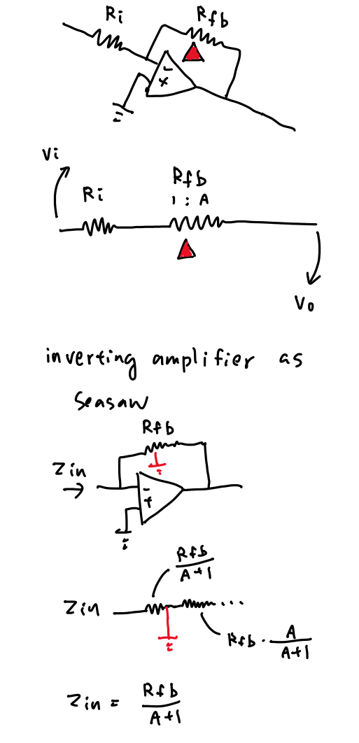
The seesaw analogy, the input resistance Zin = Rfb/(A+1), and the LHP → ∞ → RHP zero all appear in the literature — but always separately. Each source below explains one piece and drops the others. A correct input-resistance analysis is impossible without a finite gain A: the idealized (A→∞) sources can only assert a perfect virtual ground, never derive the Rfb/(A+1) node impedance this note works out.
| # | Source | What it covers well | What's missing |
|---|---|---|---|
| 1 | All About Circuits — Seesaw analogy | The lever/fulcrum intuition: virtual ground = pivot, gain = arm ratio, input down → output up. | Finite gain A — assumes an ideal (A→∞) op-amp. Therefore no input-resistance analysis, which is impossible without a finite A. Purely mechanical: no transfer function, no Miller math. |
| 2 | EDN — Miller's theorem | Rigorous split with explicit finite A: Z/(1+A) at the input, Z·A/(A+1) at the output. | The seesaw / lever intuition. Uses a generic gain block, not the OTA / transconductance (g in A/V) framing. Never links to the transmission-null / RHP-zero migration. |
| 3 | Electronics Tutorials — Virtual earth | The virtual-ground concept and closed-loop gain −Rf/Rin. | Assumes A→∞, so it just states Zin ≈ Rin and never derives the node impedance Rfb/(A+1) — the quantity that explains why it's a virtual ground. No seesaw, no Miller split. |
| 4 | All About Circuits — Miller compensation | Capacitance multiplication C·(1+A) and pole splitting for two-stage stability. | Frames it only as a capacitor for frequency comp; doesn't unify with the DC resistor Rfb/(A+1) picture. No seesaw. Doesn't show the transconductance-fed zero moving LHP → ∞ → RHP. |
| ★ | Bo's curriculum | Unifies all four: finite gain A throughout · seesaw intuition and the rigorous Zin = Rfb/(A+1) derivation · the OTA transconductance (g, A/V) model · and the interactive LHP → ∞ → RHP zero migration in this very tool. | |
📚 More derivations and interactive tools: Bo's curriculum on GitHub.