gm/Id First-Order Estimator

Interactive g_m calculator — diode-connected MOSFET

Type in W, L, id, M and the estimator computes g_m, r_o, v_ov, v_th and c_g from the first-order model on this page (diode-connected → V_ds=V_gs, saturation). Pick the model source, device type and voltage flavor below the device.

Diode-connected MOSFET biased by an id current source, source to ground; labels M, W, L, id, gm, ro, vov, vth, cg

µA

µm

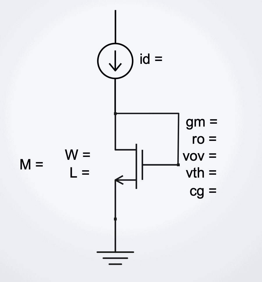
at the op-point	sim (sky130)	est (formula)
g_m	—	—
r_o	—	—
v_ov	—	—
v_th	—	—
c_g	—	—

Sim column = sky130 ngspice op-point at the operating current density (gm/I_d method, ref L=0.15 µm); only for sky130·NMOS·1.8 V. Est g_m box: dashed = weak, solid = strong inversion.

$c_g = C_{ox}\,A$

g_m vs I_d — selected device (log–log)

weak

strong

100 µm 10 µm 1 µm – – dash = weak (κ·I_d) —— solid = strong (√-law) ● op-point

sky130 curves also show the measured ngspice points (dots); other selections are the model only.

Model source

Device type

Voltage flavor

First-order saturation model: g_m=√(2·µ_nC_ox·(MW/L)·id), v_ov=2·id/g_m, r_o=1/(λid) with λ=λ′/L, c_g=C_ox·MW·L. sky130/NMOS-1.8V uses measured params (Figure 3); other combinations are first-order estimates — replace with your PDK.

Loading sketch…

Hand sketch: gm vs Ids for a 180nm NMOS, L=0.36um. eq1 gm=20*Ids (weak-inversion line), eq2 gm=1mS*sqrt(Ids/1mA)*sqrt(W/1um) (strong-inversion sqrt law), with W=10um and W=100um curves and the 250uA corner.

Figure 1 · The original bench sketch — a 180 nm NMOS, L = 0.36 µm. Everything below is a live, generalized version of it.

1. The two equations

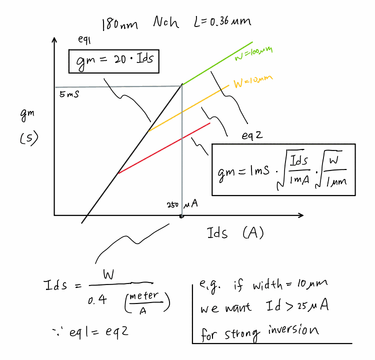
Two straight-line asymptotes bound the transconductance of a MOSFET as you sweep its drain current:

eq 1 — weak / moderate inversion (the "gm/I_d" limit)

$$g_m = \kappa\, I_d, \qquad \kappa \equiv \left(\frac{g_m}{I_d}\right)_{\max} = \frac{1}{n\,\phi_t} \approx 15\text{–}25\ \text{S/A}$$

In weak inversion the transistor behaves like a bipolar: $g_m$ is simply proportional to $I_d$, and the slope $\kappa$ is set almost entirely by physics and temperature ($\phi_t=kT/q\approx26\,\text{mV}$, subthreshold factor $n\approx1.2\text{–}1.5$) — not by the process node. The sketch uses κ = 20.

eq 2 — strong inversion (the square-law)

$$g_m = \sqrt{2\,\mu_n C_{ox}\,\frac{W}{L}\,I_d}\;=\;\underbrace{1\,\text{mS}}_{\text{sketch}}\cdot\sqrt{\frac{I_d}{1\,\text{mA}}}\cdot\sqrt{\frac{W}{1\,\mu\text{m}}}$$

Here $g_m\propto\sqrt{I_d}$, and the coefficient carries the process through $\mu_n C_{ox}$. Matching the sketch's 1 mS·√(I_d/1mA)·√(W/1µm) form at $L=0.36\,\mu\text{m}$ pins down the process constant:

$$\mu_n C_{ox} = \frac{(1\,\text{mS})^2\,L}{2}\cdot\frac{1\,\mu\text{m}}{1\,\text{mA}\cdot1\,\mu\text{m}} \;\Rightarrow\; \boxed{\mu_n C_{ox}\approx 180\ \mu\text{A/V}^2}\quad(\text{180 nm, }L=0.36\,\mu\text{m})$$

The corner — "how much current buys strong inversion"

Set eq 1 = eq 2. The two lines cross at:

$$I_{d,\text{corner}} = \frac{2\,\mu_n C_{ox}}{\kappa^2}\,\frac{W}{L},\qquad g_{m,\text{corner}}=\kappa\,I_{d,\text{corner}},\qquad \frac{I_{d,\text{corner}}}{W}=\frac{2\,\mu_n C_{ox}}{\kappa^2 L}$$

Plugging the sketch's numbers ($\mu_n C_{ox}=180\,\mu\text{A/V}^2,\ \kappa=20,\ L=0.36\,\mu\text{m}$) gives a corner current density of 2.5 µA/µm — i.e. I_d = W / 0.4 with W in µm — exactly the "if W = 10 µm we want I_d > 25 µA for strong inversion" note on the sketch. ✔

2. Live plot — g_m vs I_d

Process node

μ_nC_ox = µA/V²

κ = (g_m/I_d)_max = S/A

Channel length L = µm

Figure 2 · Transconductance g_m vs drain current I_d — the weak-inversion line meets the √-law curve

eq 1: g_m=κ·I_d (weak inv.) W = 100 µm W = 10 µm W = 1 µm ● corner (eq1 = eq2)

log–log axes (straightens both asymptotes) — default

3. Reproduced with real sky130 data (ngspice)

Figure 2 is the first-order model. Here is the real thing — an ngspice DC sweep of the open-source SkyWater sky130_fd_pr__nfet_01v8 NMOS (L = 0.15 µm, V_ds = 0.9 V, tt corner), with g_m = dI_d/dV_gs extracted at every step. Markers are sampled 4 per decade at 1 · 2.2 · 4.7 · 10, so they land evenly on the log axis. Deck + raw data in /spice.

Figure 3 · Real sky130 nfet_01v8 — g_m vs I_d (log–log), W = 1 / 10 / 100 µm

weak-inv. κ·I_d (κ≈29 S/A, real) W = 100 µm W = 10 µm W = 1 µm

Real weak-inversion slope κ = (g_m/I_d)_max ≈ 29 S/A — higher than the sketch's 20, because sky130's subthreshold factor n ≈ 1.3. Each curve hugs the κ line at low current, then rolls into the √-law region as the device enters strong inversion — exactly the shape of the hand sketch, but every point here is a simulated device, not an equation.

4. The constants vs. process node

Only one of the two constants really moves with the node. κ is temperature-limited and stays ≈ 15–25 everywhere; the process story lives in μ_nC_ox (thinner oxide raises $C_{ox}$, but scaled/strained channels change $\mu_n$) and therefore in the corner current density. The table below is seeded with rough textbook estimates — edit any cell to your PDK and both the chart and the plot update.

These are order-of-magnitude teaching numbers, not fab data. Long-channel low-field μ_nC_ox varies widely with L, V_ds, back-bias and flavor (LVT/HVT). For FinFET/GAA nodes μ_nC_ox loses its plain meaning (drive is quantized per fin) — use the gm/I_d method with your PDK LUTs there. Replace the values with your own.

Node	μ_nC_ox (µA/V²)	κ (S/A)	L_min (µm)	eq2 coeff* (mS)	corner I_d/W (µA/µm)

*eq2 coeff = the "1 mS" in g_m=coeff·√(I_d/1mA)·√(W/1µm), evaluated at that row's L_min; equals $\sqrt{2\mu_nC_{ox}\cdot(1\text{µm}/L_{min})\cdot1\text{mA}}$. Corner density uses L = L_min.

Figure 4 · First-order constants vs process node — κ (bold black, left axis) is temperature-limited and stays ≈flat; μ_nC_ox (right axis) carries the process

κ = (g_m/I_d)_max (S/A) — left μ_nC_ox (µA/V²) — right corner I_d/W at L_min (µA/µm) — left ◆ sky130 (open PDK)

5. How to use this as a design shortcut

Given a bias current, want max efficiency? Stay on the eq 1 line (weak/moderate inversion): $g_m\approx\kappa I_d$ gives the most $g_m$ per amp — great for low-power / low-noise front ends.
Given a target g_m and headroom, want speed? Push into strong inversion (eq 2). You pay current but gain $f_T$ and matching.
The corner is the design sweet spot. $I_d/W = 2\mu_nC_{ox}/(\kappa^2 L)$ tells you the minimum current density for strong inversion. Below it you're wasting $g_m$/speed; far above it you're wasting power.

Interactive gm calculator — diode-connected MOSFET