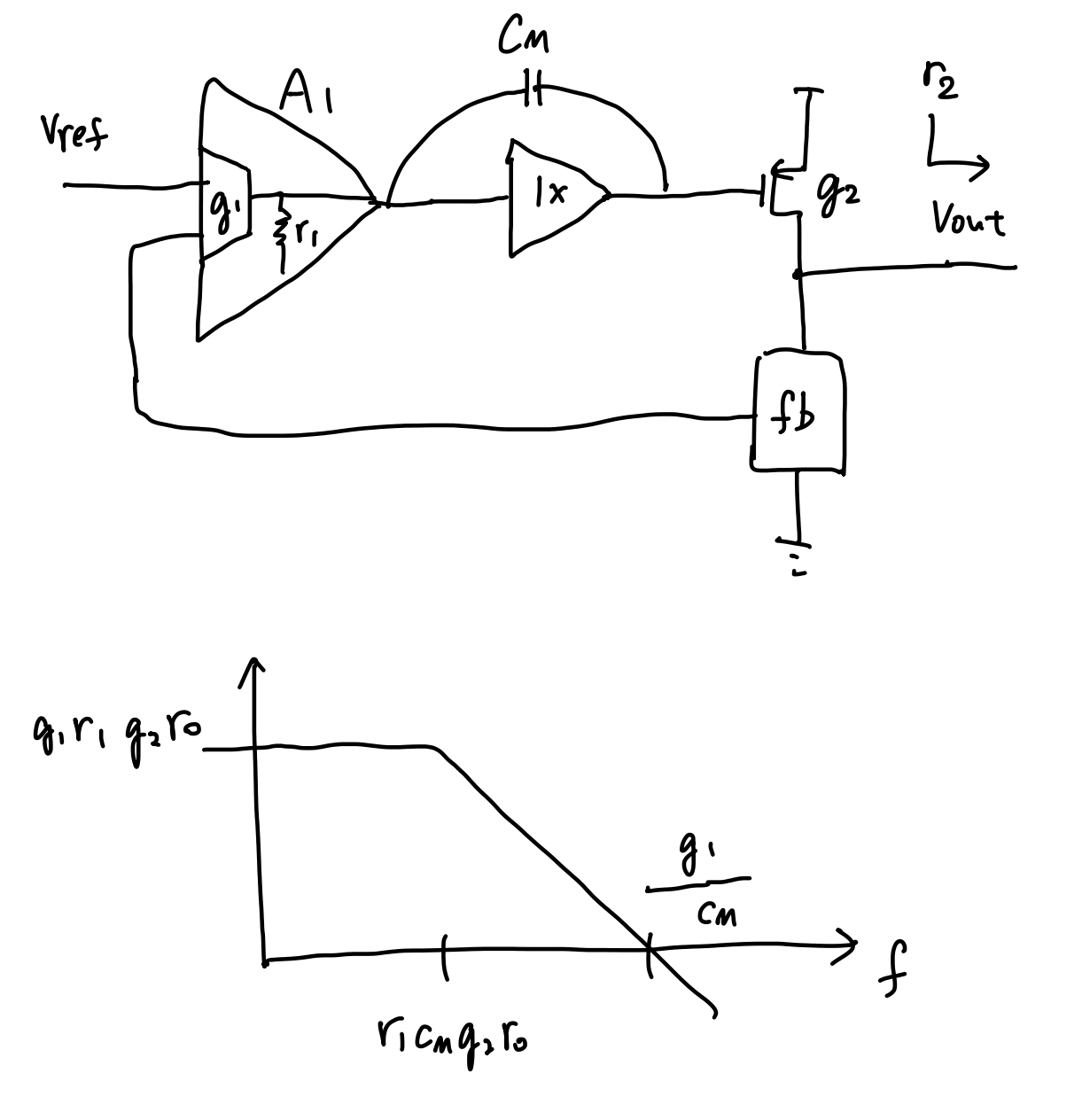
1 · Circuit & how it maps to the sketch
 Vref ─►┌─────┐        ┌─────┐        │┌───┐   ┌── Vout
        │ A₁  ├───┬────┤ 1×  ├───┬────┤│g₂ ├─┬─►
        └─────┘   │    └─────┘   │    │└───┘ │
                 (r₁)     └──[Cₘ]──────┘    (r₀‖r₂)
                                                │
        └──────────────[ fb divider ]──────────┘
Your hand sketch is a Miller-compensated two-stage amplifier: first-stage gain A₁ at node r₁, a 1× buffer that steers Cₘ (removes the RHP zero — the indirect / Ahuja style), and an output transconductor g₂ driving r₀. Loop DC gain is A₁·g₂·r₀; the Miller cap pushes the dominant pole down to 1/(2π·r₁·g₂·r₀·Cₘ), exactly the plateau + single-pole roll-off you drew.
Transistor bias table
| Device | Maps to | gm/ID | ID | gm | ro (node) |
|---|---|---|---|---|---|
| M1 — input pair | g₁ / A₁ input stage | 6.3 V⁻¹ | 15 µA | 94.25 µS | 754 kΩ (R_I) |
| M6 — output device | g₂ pass transconductor | 9.9 V⁻¹ | 95 µA | 942.5 µS | 47.5 kΩ (R_II) |
gm from Allen Ex 23-1 (§5/§7); bias currents per that example (tail I₅ = 30 µA → 15 µA/input device; I₆ ≈ 95 µA); gm/ID = gm ÷ ID; ro is the node resistance (R_I = ro2‖ro4, R_II = ro6‖ro7). The 1× buffer is a unity source-follower (no DC gain), not listed. Replace with your netlist's operating point.
2 · Interactive parameters
2.1 · Key results
2.2 · Gain-budget pie — how the loop gain splits
Total loop DC gain (in dB) is the sum of each stage's dB — so a pie of the dB contribution shows where your gain comes from.
3 · Bode plots
Magnitude |A| (dB)
Phase ∠A (deg)
4 · Ranked pole/zero table
| Rank | 📍 Singularity | Sketch label | Frequency | Position (10 Hz–1 GHz, log) |
|---|
5 · Sketch symbol → cited number
Default values recover the canonical worked example: Allen, "Design of Two-Stage Op Amps," Lecture 23, Example 23-1.
| 🔣 Sketch | Meaning | Cited value |
|---|---|---|
A₁·g₂·r₀ | DC loop gain (plateau) | 3,180 V/V = 70.0 dB |
| gm of A₁ | input g_m (gm1) | 94.25 µS |
g₂ | output g_m (gm6) | 942.5 µS |
Cₘ | Miller cap (Cc) | 3 pF |
| C_L | load cap | 10 pF |
r₁·Cₘ·g₂·r₀ | dominant pole | ≈ 1.57 kHz |
| GBW = gm1/Cₘ | unity-gain freq | 5.0 MHz |
| PM | phase margin | 60° |
6 · Transfer function & corner equations
With the 1× buffer steering Cₘ (indirect Miller), the loop gain is single-dominant-pole:
A(s) = A₁·g₂·r₀ · 1 / [ (1 + s/ω_p1)(1 + s/ω_p2) ]
| Quantity | Expression | Note |
|---|---|---|
| DC gain | A₁·g₂·r₀ | plateau height |
| Dominant pole f_p1 | 1 / (2π·r₁·g₂·r₀·Cₘ) | Miller-multiplied |
| GBW | gm1 / (2π·Cₘ) = A₁ / (2π·r₁·Cₘ) | unity-gain |
| Output pole f_p2 | g₂ / (2π·C_L) | 2nd pole |
| RHP zero f_z | g₂ / (2π·Cₘ) | only if buffer OFF |
g₂/(2π·Cₘ). Toggle the buffer off to see that zero reappear and flatten the phase roll-off (degrading PM).7 · Sources & citation
Primary (default values): P. E. Allen, "CMOS Analog Circuit Design — Lecture 23: Design of Two-Stage Op Amps," Example 23-1. A_v = 3,180 V/V (70 dB), GB = 5 MHz, PM = 60°, Cc = 3 pF, C_L = 10 pF, gm1 = 94.25 µS, gm6 = 942.5 µS. aicdesign.org/…/lecture23-160311.pdf
Buffered / indirect Miller (matches the 1× buffer): Manoj et al., "Miller's Compensation Techniques for a High Gain, High BW Two-Stage Op-Amp," N-Publications, 2022 — A₀ = 77.7 dB, GBW = 110 MHz, PM = 60°, Cₘ = 20 pF, C_L = 100 pF, 65 nm, ±1.5 V. npublications.com/…/c242005-110(2022).pdf
Mechanism / independent worked example: All About Circuits, "Miller Frequency Compensation" — Cf = 9.9 pF, dominant pole 63.4 Hz, 2nd pole 12.2 MHz, PM 65.5°. allaboutcircuits.com/…/miller-frequency-compensation
Spec-target reference: TAMU ECEN 474 Lab 8 — Two-Stage Miller Op-Amp. people.engr.tamu.edu/spalermo/ecen474/Lab8.pdf